Introduction to Pandas in Python¶

Estimated time needed: 15 minutes

Objectives¶

After completing this lab you will be able to:

• Use Pandas to access and view data

Table of Contents

• About the Dataset
• Introduction of Pandas
• Viewing Data and Accessing Data
• Quiz on DataFrame

---

About the Dataset

The table has one row for each album and several columns.

• artist: Name of the artist
• album: Name of the album
• released_year: Year the album was released
• length_min_sec: Length of the album (hours,minutes,seconds)
• genre: Genre of the album
• music_recording_sales_millions: Music recording sales (millions in USD) on [SONG://DATABASE]
• claimed_sales_millions: Album's claimed sales (millions in USD) on [SONG://DATABASE]
• date_released: Date on which the album was released
• soundtrack: Indicates if the album is the movie soundtrack (Y) or (N)
• rating_of_friends: Indicates the rating from your friends from 1 to 10

You can see the dataset here:

Artist	Album	Released	Length	Genre	Music recording sales (millions)	Claimed sales (millions)	Released	Soundtrack	Rating (friends)
Michael Jackson	Thriller	1982	00:42:19	Pop, rock, R&B	46	65	30-Nov-82		10.0
AC/DC	Back in Black	1980	00:42:11	Hard rock	26.1	50	25-Jul-80		8.5
Pink Floyd	The Dark Side of the Moon	1973	00:42:49	Progressive rock	24.2	45	01-Mar-73		9.5
Whitney Houston	The Bodyguard	1992	00:57:44	Soundtrack/R&B, soul, pop	26.1	50	25-Jul-80	Y	7.0
Meat Loaf	Bat Out of Hell	1977	00:46:33	Hard rock, progressive rock	20.6	43	21-Oct-77		7.0
Eagles	Their Greatest Hits (1971-1975)	1976	00:43:08	Rock, soft rock, folk rock	32.2	42	17-Feb-76		9.5
Bee Gees	Saturday Night Fever	1977	1:15:54	Disco	20.6	40	15-Nov-77	Y	9.0
Fleetwood Mac	Rumours	1977	00:40:01	Soft rock	27.9	40	04-Feb-77		9.5

---

Introduction of Pandas

In [1]:

# Dependency needed to install file 

!pip install xlrd

# Dependency needed to install file !pip install xlrd

Requirement already satisfied: xlrd in /home/jupyterlab/conda/envs/python/lib/python3.7/site-packages (1.2.0)

In [2]:

# Import required library

import pandas as pd

# Import required library import pandas as pd

After the import command, we now have access to a large number of pre-built classes and functions. This assumes the library is installed; in our lab environment all the necessary libraries are installed. One way pandas allows you to work with data is a dataframe. Let's go through the process to go from a comma separated values (.csv) file to a dataframe. This variable csv_path stores the path of the .csv, that is used as an argument to the read_csv function. The result is stored in the object df, this is a common short form used for a variable referring to a Pandas dataframe.

In [3]:

# Read data from CSV file

csv_path = 'https://cf-courses-data.s3.us.cloud-object-storage.appdomain.cloud/IBMDeveloperSkillsNetwork-PY0101EN-SkillsNetwork/labs/Module%204/data/TopSellingAlbums.csv'
df = pd.read_csv(csv_path)

# Read data from CSV file csv_path = 'https://cf-courses-data.s3.us.cloud-object-storage.appdomain.cloud/IBMDeveloperSkillsNetwork-PY0101EN-SkillsNetwork/labs/Module%204/data/TopSellingAlbums.csv' df = pd.read_csv(csv_path)

We can use the method head() to examine the first five rows of a dataframe:

In [4]:

# Print first five rows of the dataframe

df.head()

# Print first five rows of the dataframe df.head()

Out[4]:

	Artist	Album	Released	Length	Genre	Music Recording Sales (millions)	Claimed Sales (millions)	Released.1	Soundtrack	Rating
0	Michael Jackson	Thriller	1982	0:42:19	pop, rock, R&B	46.0	65	30-Nov-82	NaN	10.0
1	AC/DC	Back in Black	1980	0:42:11	hard rock	26.1	50	25-Jul-80	NaN	9.5
2	Pink Floyd	The Dark Side of the Moon	1973	0:42:49	progressive rock	24.2	45	01-Mar-73	NaN	9.0
3	Whitney Houston	The Bodyguard	1992	0:57:44	R&B, soul, pop	27.4	44	17-Nov-92	Y	8.5
4	Meat Loaf	Bat Out of Hell	1977	0:46:33	hard rock, progressive rock	20.6	43	21-Oct-77	NaN	8.0

We use the path of the excel file and the function read_excel. The result is a data frame as before:

In [5]:

# Read data from Excel File and print the first five rows

xlsx_path = 'https://s3-api.us-geo.objectstorage.softlayer.net/cf-courses-data/CognitiveClass/PY0101EN/Chapter%204/Datasets/TopSellingAlbums.xlsx'

df = pd.read_excel(xlsx_path)
df.head()

# Read data from Excel File and print the first five rows xlsx_path = 'https://s3-api.us-geo.objectstorage.softlayer.net/cf-courses-data/CognitiveClass/PY0101EN/Chapter%204/Datasets/TopSellingAlbums.xlsx' df = pd.read_excel(xlsx_path) df.head()

---------------------------------------------------------------------------
ImportError                               Traceback (most recent call last)
/tmp/ipykernel_68/2455837228.py in <module>
      3 xlsx_path = 'https://s3-api.us-geo.objectstorage.softlayer.net/cf-courses-data/CognitiveClass/PY0101EN/Chapter%204/Datasets/TopSellingAlbums.xlsx'
      4 
----> 5 df = pd.read_excel(xlsx_path)
      6 df.head()

~/conda/envs/python/lib/python3.7/site-packages/pandas/util/_decorators.py in wrapper(*args, **kwargs)
    309                     stacklevel=stacklevel,
    310                 )
--> 311             return func(*args, **kwargs)
    312 
    313         return wrapper

~/conda/envs/python/lib/python3.7/site-packages/pandas/io/excel/_base.py in read_excel(io, sheet_name, header, names, index_col, usecols, squeeze, dtype, engine, converters, true_values, false_values, skiprows, nrows, na_values, keep_default_na, na_filter, verbose, parse_dates, date_parser, thousands, comment, skipfooter, convert_float, mangle_dupe_cols, storage_options)
    362     if not isinstance(io, ExcelFile):
    363         should_close = True
--> 364         io = ExcelFile(io, storage_options=storage_options, engine=engine)
    365     elif engine and engine != io.engine:
    366         raise ValueError(

~/conda/envs/python/lib/python3.7/site-packages/pandas/io/excel/_base.py in __init__(self, path_or_buffer, engine, storage_options)
   1231         self.storage_options = storage_options
   1232 
-> 1233         self._reader = self._engines[engine](self._io, storage_options=storage_options)
   1234 
   1235     def __fspath__(self):

~/conda/envs/python/lib/python3.7/site-packages/pandas/io/excel/_openpyxl.py in __init__(self, filepath_or_buffer, storage_options)
    519             passed to fsspec for appropriate URLs (see ``_get_filepath_or_buffer``)
    520         """
--> 521         import_optional_dependency("openpyxl")
    522         super().__init__(filepath_or_buffer, storage_options=storage_options)
    523 

~/conda/envs/python/lib/python3.7/site-packages/pandas/compat/_optional.py in import_optional_dependency(name, extra, errors, min_version)
    116     except ImportError:
    117         if errors == "raise":
--> 118             raise ImportError(msg) from None
    119         else:
    120             return None

ImportError: Missing optional dependency 'openpyxl'.  Use pip or conda to install openpyxl.

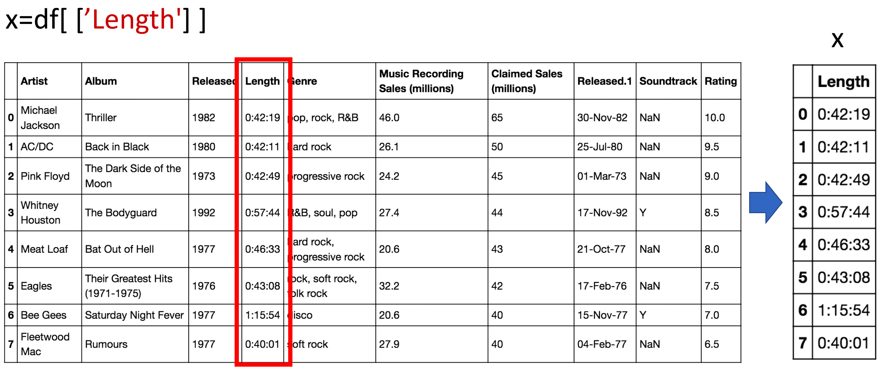
We can access the column Length and assign it a new dataframe x:

In [6]:

# Access to the column Length

x = df[['Length']]
x

# Access to the column Length x = df[['Length']] x

Out[6]:

	Length
0	0:42:19
1	0:42:11
2	0:42:49
3	0:57:44
4	0:46:33
5	0:43:08
6	1:15:54
7	0:40:01

The process is shown in the figure:

---

Viewing Data and Accessing Data

You can also get a column as a series. You can think of a Pandas series as a 1-D dataframe. Just use one bracket:

In [7]:

# Get the column as a series

x = df['Length']
x

# Get the column as a series x = df['Length'] x

Out[7]:

0    0:42:19
1    0:42:11
2    0:42:49
3    0:57:44
4    0:46:33
5    0:43:08
6    1:15:54
7    0:40:01
Name: Length, dtype: object

You can also get a column as a dataframe. For example, we can assign the column Artist:

In [8]:

# Get the column as a dataframe

x = df[['Artist']]
type(x)

# Get the column as a dataframe x = df[['Artist']] type(x)

Out[8]:

pandas.core.frame.DataFrame

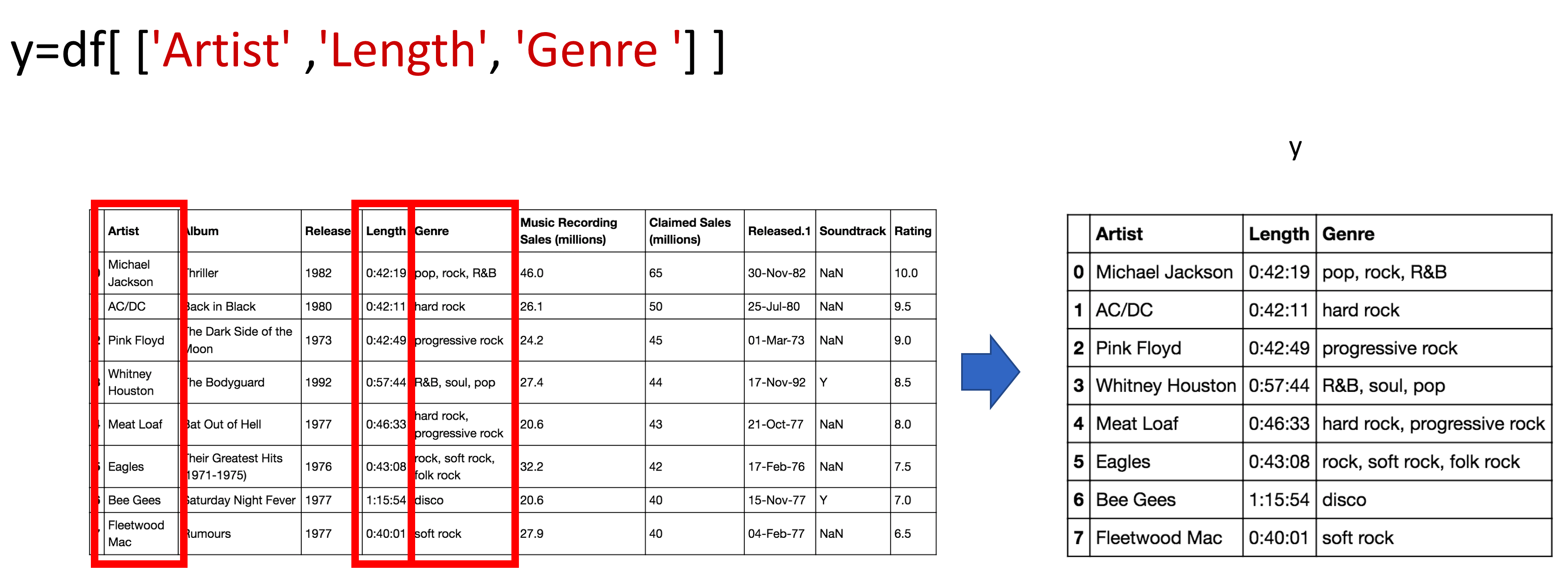
You can do the same thing for multiple columns; we just put the dataframe name, in this case, df, and the name of the multiple column headers enclosed in double brackets. The result is a new dataframe comprised of the specified columns:

In [9]:

# Access to multiple columns

y = df[['Artist','Length','Genre']]
y

# Access to multiple columns y = df[['Artist','Length','Genre']] y

Out[9]:

	Artist	Length	Genre
0	Michael Jackson	0:42:19	pop, rock, R&B
1	AC/DC	0:42:11	hard rock
2	Pink Floyd	0:42:49	progressive rock
3	Whitney Houston	0:57:44	R&B, soul, pop
4	Meat Loaf	0:46:33	hard rock, progressive rock
5	Eagles	0:43:08	rock, soft rock, folk rock
6	Bee Gees	1:15:54	disco
7	Fleetwood Mac	0:40:01	soft rock

The process is shown in the figure:

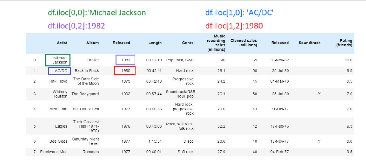
One way to access unique elements is the iloc method, where you can access the 1st row and the 1st column as follows:

In [10]:

# Access the value on the first row and the first column

df.iloc[0, 0]

# Access the value on the first row and the first column df.iloc[0, 0]

Out[10]:

'Michael Jackson'

You can access the 2nd row and the 1st column as follows:

In [11]:

# Access the value on the second row and the first column

df.iloc[1,0]

# Access the value on the second row and the first column df.iloc[1,0]

Out[11]:

'AC/DC'

You can access the 1st row and the 3rd column as follows:

In [12]:

# Access the value on the first row and the third column

df.iloc[0,2]

# Access the value on the first row and the third column df.iloc[0,2]

Out[12]:

1982

In [13]:

# Access the value on the second row and the third column
df.iloc[1,2]

# Access the value on the second row and the third column df.iloc[1,2]

Out[13]:

1980

In [ ]:

This is shown in the following image

You can access the column using the name as well, the following are the same as above:

In [14]:

# Access the column using the name

df.loc[1, 'Artist']

# Access the column using the name df.loc[1, 'Artist']

Out[14]:

'AC/DC'

In [15]:

# Access the column using the name

df.loc[1, 'Artist']

# Access the column using the name df.loc[1, 'Artist']

Out[15]:

'AC/DC'

In [16]:

# Access the column using the name

df.loc[0, 'Released']

# Access the column using the name df.loc[0, 'Released']

Out[16]:

1982

In [17]:

# Access the column using the name

df.loc[1, 'Released']

# Access the column using the name df.loc[1, 'Released']

Out[17]:

1980

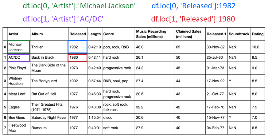
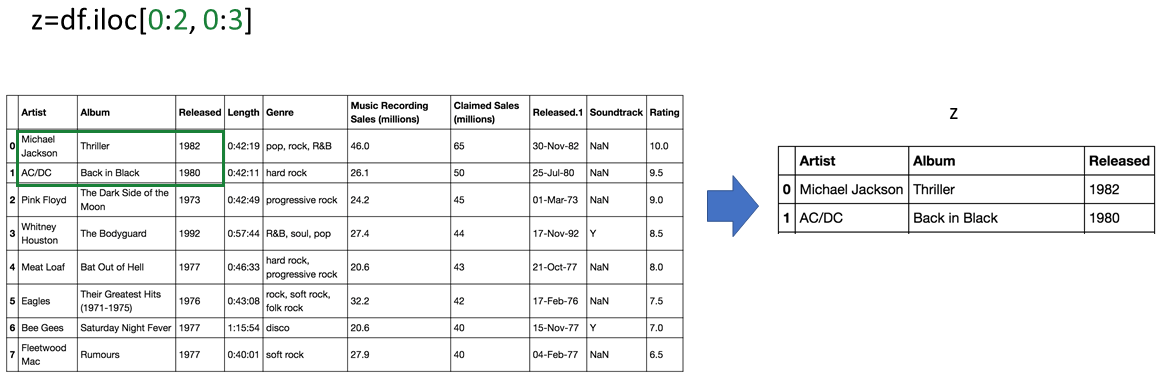
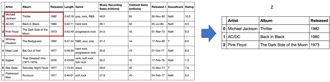
You can perform slicing using both the index and the name of the column:

In [18]:

# Slicing the dataframe

df.iloc[0:2, 0:3]

# Slicing the dataframe df.iloc[0:2, 0:3]

Out[18]:

	Artist	Album	Released
0	Michael Jackson	Thriller	1982
1	AC/DC	Back in Black	1980

In [19]:

# Slicing the dataframe using name

df.loc[0:2, 'Artist':'Released']

# Slicing the dataframe using name df.loc[0:2, 'Artist':'Released']

Out[19]:

	Artist	Album	Released
0	Michael Jackson	Thriller	1982
1	AC/DC	Back in Black	1980
2	Pink Floyd	The Dark Side of the Moon	1973

---

Quiz on DataFrame

Use a variable q to store the column Rating as a dataframe

In [22]:

# Write your code below and press Shift+Enter to execute
q = df[['Rating']]
q

# Write your code below and press Shift+Enter to execute q = df[['Rating']] q

Out[22]:

	Rating
0	10.0
1	9.5
2	9.0
3	8.5
4	8.0
5	7.5
6	7.0
7	6.5

Click here for the solution

q = df[['Rating']]
q
    

Assign the variable q to the dataframe that is made up of the column Released and Artist:

In [26]:

# Write your code below and press Shift+Enter to execute
q = df[['Released', 'Artist']]
q

# Write your code below and press Shift+Enter to execute q = df[['Released', 'Artist']] q

Out[26]:

	Released	Artist
0	1982	Michael Jackson
1	1980	AC/DC
2	1973	Pink Floyd
3	1992	Whitney Houston
4	1977	Meat Loaf
5	1976	Eagles
6	1977	Bee Gees
7	1977	Fleetwood Mac

Click here for the solution

q = df[['Released', 'Artist']]
q
    

Access the 2nd row and the 3rd column of df:

In [28]:

# Write your code below and press Shift+Enter to execute
df.iloc[1:2]

# Write your code below and press Shift+Enter to execute df.iloc[1:2]

Out[28]:

	Artist	Album	Released	Length	Genre	Music Recording Sales (millions)	Claimed Sales (millions)	Released.1	Soundtrack	Rating
1	AC/DC	Back in Black	1980	0:42:11	hard rock	26.1	50	25-Jul-80	NaN	9.5

Click here for the solution

df.iloc[1, 2]
    

Use the following list to convert the dataframe index df to characters and assign it to df_new; find the element corresponding to the row index a and column 'Artist'. Then select the rows a through d for the column 'Artist'

In [35]:

new_index=['a','b','c','d','e','f','g','h']
df_new = df
df_new.index = new_index
df_new.loc['a', 'Artist']
df_new.loc['a':'d', 'Artist']

new_index=['a','b','c','d','e','f','g','h'] df_new = df df_new.index = new_index df_new.loc['a', 'Artist'] df_new.loc['a':'d', 'Artist']

Out[35]:

a    Michael Jackson
b              AC/DC
c         Pink Floyd
d    Whitney Houston
Name: Artist, dtype: object

Click here for the solution

df_new=df
df_new.index=new_index
df_new.loc['a', 'Artist']
df_new.loc['a':'d', 'Artist']
    

---

The last exercise!

Congratulations, you have completed your first lesson and hands-on lab in Python.

---

Authors:¶

Joseph Santarcangelo

Joseph Santarcangelo has a PhD in Electrical Engineering, his research focused on using machine learning, signal processing, and computer vision to determine how videos impact human cognition. Joseph has been working for IBM since he completed his PhD.

Change Log¶

Date (YYYY-MM-DD)	Version	Changed By	Change Description
2022-01-10	2.1	Malika	Removed the readme for GitShare
2020-08-26	2.0	Lavanya	Moved lab to course repo in GitLab
2020-11-24	3.0	Nayef	Added new images

---

© IBM Corporation 2020. All rights reserved.